How often do we as researchers want to attribute causality to what we know is just correlational? It can be so easy to mix up correlation with causation! And in our industry we do driver analyses so often. The mix-up is easy: for example, ice cream sales and drownings both increase during summer, but it doesn’t mean that one causes the other.
Correlation shows that variables change together. Causation explains which variable leads to the change in the other, and this is very important when deciding where to invest or which factors really have the effect.
This distinction becomes especially important in advanced analytics approaches, where decisions depend on identifying true drivers rather than coincidental patterns.
The Analytics Team has been finding causal drivers for over 7 years now applying cutting-edge validated methods. And we have built interactive maps and simulators around these leading insights. These take typical drivers to the next level of practical application. This is a short “beginners” guide to what we are doing and how we do it. It gets a little deep so we won’t judge if you skip/skim some sections!
Why Causal Inference Matters
Causal inference tells us what the effect on Y would be if we changed X. The problem is, traditional analytics just can’t figure this out. Correlation doesn’t explain whether changing X really causes Y, or the two are being driven by some other factor.
Causal Inference vs. Causal Discovery
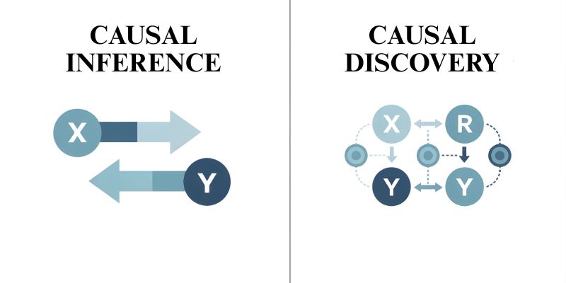
Causal inference: is a method of testing a hypothesis. You think that X gives rise to Y and want to find out by how much. For example, do sales go up if we run this campaign? The framework is given beforehand. You’re measuring the impact.
Causal discovery: is going in the reverse direction. You’re not aware of which variables are the causes and which are the effects. You possess the data, and you want to understand the causal structure from it. For instance, in a given system, what is the cause and what is the effect? Discovery identifies the connections. Inference evaluates them.
The Causal Methods Landscape
Constraint-based methods: like the PC test conditional independence. They figure out which variables are independent of others and create graphs based on those patterns. They are flexible but require large samples.
Score-based methods: they rate various structures and choose the one that fits best. They handle noise better but are computationally expensive.
Functional causal models: suppose specific mathematical relationships. LiNGAM is one of them. These use the property of the relationships to find the causal direction.
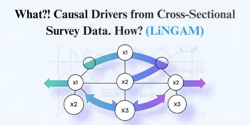
What Is LiNGAM?
LiNGAM (Linear Non-Gaussian Acyclic Model) reveals the entire causal network, including direction, solely from observational data. What sets LiNGAM apart is its ability, under specific conditions, to identify which variable causes the other, not just that a relationship exists. In contrast, most other methods can only narrow the possibilities to equivalent structures, leaving the causal direction ambiguous.
Why LiNGAM Exists and What Makes It Different
One of the main limitations of traditional methods is that different causal structures can give rise to the same statistical patterns; thus, the methods fail to distinguish one from another. For instance, it is impossible to identify which one is causing the other, X causing Y or Y causing X, just from looking at the correlations.
LiNGAM gets to the root of the problem: if the relationships between variables are linear and those errors or noise are non, Gaussian, the direction of causality can be determined.
It employs Independent Component Analysis to separate the data into independent noise parts, and then it finds the order of causality. Unlike PC, which can give several causal structures, LiNGAM provides one specific directed graph.
Key Assumptions and Why They Matter
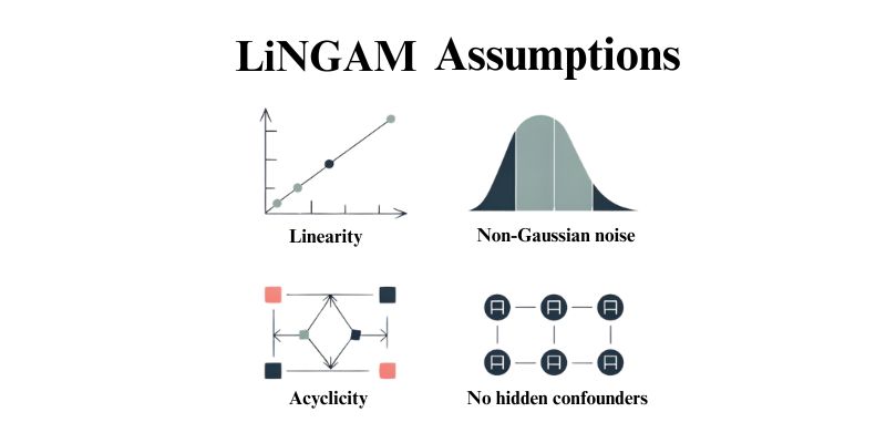
Linearity: Variables are related in straight line patterns only. An exponential growth or the presence of a threshold can change this.
Non-Gaussian noise: The random errors cannot be normally distributed. This allows one to find out the direction.
Acyclicity: The graph or network has no cycles or feedback loops. A causes B, causes C, but C can’t cause A. Time series extensions allow the handling of autoregressive effects.
No hidden confounders: All common causes must be observed. The presence of unmeasured variables will lead to errors. Variants like RCD deal with confounding to some extent.
These set the boundary for the success and failure of LiNGAM.
How LiNGAM Works Conceptually
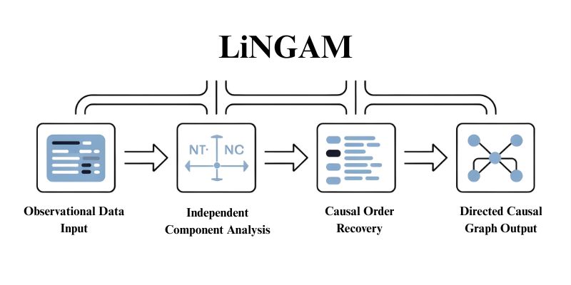
Given that the relationships are linear and the noise is non-Gaussian, the observed data consist of mixtures of independent components of noise from each causal equation.
To separate the components, LiNGAM applies Independent Component Analysis on the data. Non-Gaussianity guarantees that only one unmixing results in genuinely independent components.
The procedure first recovers the causal order, then estimates the strength of the relationships, and finally produces a directed causal graph.
Use Cases and Practical Considerations
LiNGAM performs very well on continuous measurements where the relationships are linear: examples are healthcare pathways, market indicators, production metrics, and marketing attribution.
Strengths: How the different parts of a causal system interact with each other can be understood completely from observational data alone without needing to do any experiments. In addition, it is fast.
Limitations: To work properly, very tight assumptions must be made. If any of the nonlinear relationships, Gaussian noise, feedback loops, or confounders are present, the method will not work. Also, it needs a sufficient number of samples, and if some variables are not measured, the results will be biased.
Common Mistakes
- Ignoring assumptions. Test for non-Gaussianity and nonlinear patterns.
- Trusting outputs blindly. Validate against domain knowledge.
- Insufficient data. Small samples yield unstable results.
- Expecting perfection. Treat outputs as hypotheses.
Comparison with Other Methods
PC algorithm: Works with Gaussian data and discrete variables. Provides only graph equivalence classes, not definite unique directions. Often preferable for mixed cases when ambiguous directions are acceptable.
Granger causality: Applicable to time series. Examines the statistical association between X’s past and Y’s present. More straightforward, but it doesn’t ensure real causation.
Experiments: The best if you can do them. Apply discovery methods when experiments are not an option.
Choosing the Right Approach
Continuous data, linear relationships, non-Gaussian noise, no feedback, no confounders: LiNGAM.
Gaussian noise or discrete variables: PC.
Time series with feedback: VAR-LiNGAM.
Hidden confounders: FCI or RCD.
Experiments possible: Run them.
The Bottom Line
At the Analytics Team, causal discovery methods like LiNGAM are used not as black-box solutions, but as disciplined tools to uncover real drivers behind business outcomes. When applied carefully—respecting assumptions, validating against domain knowledge, and combining discovery with inference—these methods help organizations move beyond surface-level correlations toward decisions grounded in cause and effect.
Causal insights are most powerful when they inform strategy, experimentation, and execution together. Discovery generates hypotheses; inference and validation turn them into action. Used this way, causal analytics becomes a practical asset rather than a theoretical exercise.
If you’d like to explore how LiNGAM or other causal inference approaches can support your analytics initiatives, schedule a free 30-minute consultation call with the Analytics Team. We’ll help you determine the right method for your data, goals, and decision context.